Time Series
Foundation Models

The "ChatGPT moment" for forecasting?


Alessandro Romano

Alessandro Romano

Alessandro Romano

Data Scientist • Musician • Public Speaker

Senior Data Scientist at Kuehne+Nagel in Hamburg. 7+ years building ML & LLM solutions for pricing and forecasting.

M.Sc. Data Science, Pisa | Cargonexx → FREE NOW → Kuehne+Nagel

www.aromano.dev

Agenda

1 Time Series Is Everywhere
2 How We Do Time Series Today
3 The Transformer Revolution
4 Foundation Models for Time Series
5 Live Demo — ARIMA vs Chronos vs TimesFM
6 Challenges & When to Use
7 Takeaways & Q&A

Time Series Is Everywhere

You already work with time series

Any measurement recorded over time is a time series. They show up in virtually every industry:

Finance stock prices, risk metrics Climate temperature, CO2, precipitation IoT Sensors telemetry, device readings Energy grid load, demand, solar output Healthcare ECG, SpO2, heart rate Retail sales, inventory, foot traffic Tech web traffic, API latency, errors UCL LCL Manufacturing quality control, vibration, yield

If your data has a timestamp column, you're doing time series analysis — whether you call it that or not.

What do we do with them?

Four core tasks show up again and again across domains:

  • Forecasting — predict future values (e.g. next week's energy demand, next quarter's revenue)
  • Anomaly detection — spot outliers in real time (e.g. fraud, equipment failure, network intrusion)
  • Classification — label a pattern (e.g. is this ECG normal or arrhythmic? is this sensor vibration a bearing fault?)
  • Imputation — fill in missing data (e.g. sensor went offline for 2 hours, reconstruct what happened)

Today, each of these tasks — for each dataset — requires building and training a separate model from scratch. That's about to change.

Key properties of time series

Before modelling, you need to understand the structure of your data.

Stationarity stationary non-stationary The data "behaves the same" no matter when you look at it. e.g. room temperature with AC on vs. a stock price drifting up Autocorrelation lag 1 lag 8 Today's value depends on its own past values. e.g. if today is hot, tomorrow is likely hot too Seasonality 1 period Repeating patterns at fixed intervals (daily, weekly, yearly). e.g. ice cream sales spike every summer Trend Long-term upward or downward direction in the data. e.g. global CO2 levels rising steadily since the 1950s

Anatomy of a time series

Original = Trend × Seasonality × Residuals

Original = Trend × Seasonality × Residuals  (multiplicative decomposition)

How We Do It Today

50 years of progress — and the same pain points

The evolution of time series modeling

ARIMA Statistical forecasting 1970s RNNs Sequential neural nets 1986 LSTMs Memory gates long sequences 1997 Transformers Self-attention parallelizable 2017 GPT / BERT LLM revolution in text 2018-19 Time Series FMs Foundation models for temporal data 2023-24 handled non-linearity learned long-term memory parallel + long-range pre-train once, scale apply to time series

Classical: ARIMA & friends

The workhorse of statistical forecasting since the 1970s. Models time series as three combined components:

AR
AutoRegressive
Future depends on its own past values
trend removed I
Integrated (Differencing)
Remove trends to make data stationary
err err MA
Moving Average
Correct using past forecast errors
Strengths: interpretable coefficients, fast to fit, well-understood theory, works great for simple stationary data with clear seasonality
Limitations: assumes stationarity, needs domain knowledge (season_length, log transforms), struggles with non-linearity, can't transfer across datasets

Machine Learning & Deep Learning eras

ML: XGBoost, LightGBM raw data lag_7d rolling_30d day_of_week tree model Handles non-linear patterns well Dominated forecasting competitions You must hand-craft every feature lags, rolling stats, calendar flags — different for every dataset Effort: ~80% feature engineering modeling DL: RNNs → LSTMs raw data h1 h2 h3 h4 sequential cells Learns sequences end-to-end No feature engineering needed Memory gates retain long-term patterns Sequential = slow & can't parallelize Still struggle with very long-range dependencies (1000s of steps) Effort: data architecture + training GPU compute Both are improvements — but both still require training from scratch for every dataset.

The real pain across all these approaches

Every new dataset = train a new model from scratch

Whether you use ARIMA, XGBoost, or LSTMs, the workflow is the same: collect data, engineer features, select a model, tune hyperparameters, train, evaluate, deploy. Then a new site, a new region, or a new metric comes along — and you repeat the entire process.


New Dataset Site A, Region 1 Collect Data Feature Engineering Model Selection Hyperparam Tuning Train Model Evaluate Deploy New site? REPEAT ALL New Dataset Site B, Region 2 Collect Data Feature Eng... ...

The Transformer Revolution

The architecture behind ChatGPT — and now, time series

2017: "Attention Is All You Need"

Core idea: self-attention — every position looks at all other positions at once.

RNN: sequential

The cat sat on step 1 step 2 step 3 step 4 One at a time. Slow. "sat" barely remembers "The"

Transformer: all at once

The cat sat on All at once. Parallel. Every word "sees" every other

Under the hood: from text to predictions

An LLM processes text through a pipeline. Let's trace "The cat sat on the ___":

1. Tokenize Split text into sub-word pieces The cat sat on the vocab of ~50k tokens (not characters!) 2. Embed Each token → a vector "The" "cat" "sat" position in "meaning space" (768+ dims) 3. Self-Attention Each token asks: "who matters to me?" The cat sat on the "cat" + "sat" get high attention for predicting ___ 4. Stack & Repeat 12 to 96 transformer layers attention + feed-forward attention + feed-forward attention + feed-forward each layer refines understanding 5. Predict next token: probability over entire vocabulary mat — 62% rug — 8% floor — 6% bed — 4% ... 50,000 tokens ranked Sample from this distribution = why LLMs can give different answers each time Training = adjust weights to get better at this prediction Feed it trillions of tokens from books, web, code, Wikipedia. Repeat billions of times. Each step: predict next token, compare with actual, update weights.

The surprising power of next-token prediction

To predict the next word well, the model must learn about the world:

"The capital of France is ___"
Requires geography
"If x = 3 and y = 7, then x + y = ___"
Requires arithmetic
"def fibonacci(n):___"
Requires coding
"She smiled but her eyes looked ___"
Requires emotional reasoning
The insight: "Predict the next token" sounds trivial. But at scale, it forces the model to build an internal representation of grammar, facts, logic, and common sense — as a side effect of getting better at prediction.

This is the "foundation model" paradigm: train once on a massive general objective, then apply to specific tasks. Can we do the same for time series?

Foundation Models
for Time Series

The concept, the architecture, and the players

The two-stage paradigm

The same idea behind LLMs, applied to time series: learn general patterns first, then choose your path.

1. Pre-training Goal: learn the "language" of time series What it sees: Millions of series from diverse domains — energy, retail, weather, finance, health... What it learns: "Seasonality repeats" "Trends continue" "Spikes are temporary" Expensive (done once by Google, Amazon, etc.) You download the result for free 2a. Zero-shot Use the model directly — no training at all How: Feed your raw data in, get predictions out. No labels, no setup, no GPU needed. Works well when your data resembles training distribution. 2b. Fine-tuning Adapt the model to your domain How: Retrain on a small sample of your data. Full fine-tune, LoRA, or frozen backbone + head. Best when your domain is niche or zero-shot isn't enough. Analogy: Medical student learns general medicine (anatomy, pharmacology) then either works in any hospital immediately (zero-shot) or specializes in cardiology (fine-tuning).

"Foundation-al" = one model, many tasks

Pre-trained Foundation Model Trained on billions of diverse time points Forecasting energy demand, sales Anomaly Detection sensor outliers, fraud Classification activity, diagnosis Imputation fill sensor gaps Generation synthetic data, augment Each task via zero-shot or fine-tuning — same backbone Precedent: IBM-NASA geospatial FM — one model for floods, crops, wildfires

But how do you feed a time series to a transformer?

Transformers were built for text — sequences of discrete words. Time series are continuous signals with no natural token boundaries.

What a transformer expects Token Token Token Token Discrete, bounded, countable ? What time series looks like Continuous, no boundaries, infinite precision The core engineering challenge How do you turn a continuous signal into discrete tokens? Two approaches emerged: bin the values (Chronos) or group into patches (TimesFM)

The key insight

Text "The cat sat on the mat" The cat sat on the mat Words are natural tokens Time Series [112, 118, 132, 129, 121, 135...] No natural boundaries! vs Two solutions emerged: Chronos: Tokenization Bin continuous values into discrete tokens 18.3 → bin #42    19.1 → bin #44 Then feed tokens to a T5 language model TimesFM: Patching Group 32 values into "patches" (mini-windows) [v1...v32] → Patch 1    [v33...v64] → Patch 2 Each patch becomes one token for the transformer

Chronos: Tokenization & Embedding

Bin continuous values into discrete tokens — then each token is looked up in a learned embedding table, exactly like word embeddings in GPT.

1. Raw values 18.3 19.1 22.7 21.5 quantize 2. Bin IDs (tokens) #42 #44 #55 #51 lookup 3. Embedding vectors v₄₂ [0.18, -0.41,…] v₄₄ [0.19, -0.39,…] v₅₅ [0.74, 0.22,…] v₅₁ [0.61, 0.15,…] 4. T5 transformer self-attention on vectors 5. Predicted bins #48 #53 20.1 22.0 decode back The embedding lookup — identical mechanism to LLM word embeddings Chronos: bin ID → vector #41 → [ 0.17, -0.42, 0.71, … ] #42 → [ 0.18, -0.41, 0.72, … ] #43 → [ 0.19, -0.40, 0.73, … ] #44 → [ 0.19, -0.39, 0.74, … ] Vocabulary: 4096 quantization bins Neighboring bins → similar vectors learned: values 18.3 and 18.4 sit close in vector space GPT: word token → vector "cat" → [ 0.45, 0.12, -0.33, … ] "kitten" → [ 0.46, 0.13, -0.32, … ] "dog" → [ 0.44, 0.15, -0.30, … ] "car" → [-0.21, 0.63, 0.08, … ] Vocabulary: ~50k words/subwords Similar meaning → similar vectors cat and kitten are close; car is far away

The embedding captures meaning

A learned embedding is a map of meaning: tokens that mean similar things sit close together — words in GPT, numbers in Chronos.

GPT: word embedding space royalty king queen people man woman fruit apple banana pear similar meaning → close in space Chronos: bin embedding space values ~35 #88 #89 values ~18 #42 #43 #44 values ~10 #20 #22 similar value → close in space Chronos learns the geometry of numbers, the way GPT learns the geometry of words

TimesFM: Patching

Group 32 consecutive values into "patches" — like reading word-by-word instead of letter-by-letter. Each patch captures local patterns; attention connects them globally. Same idea as Vision Transformers (ViT).

Vision Transformer (ViT) P1 P2 P3 P4 Split image into 4×4 grid Each patch = one "token" Same idea! TimesFM (Patching) Patch 1 Patch 2 Patch 3 Patch 4 32 values Split series into fixed-length windows Each patch = one "token"

The paradigm shift

Before: one model per task per dataset Dataset A Dataset B Dataset C Dataset D Forecast Anomaly Classify Impute modelmodel modelmodel modelmodel modelmodel modelmodel modelmodel modelmodel modelmodel 16 separate models After: one backbone + task heads Foundation Model Pre-trained once Forecast Anomaly Classify Impute Works on Dataset A, B, C, D... ...and any new dataset (zero-shot) 1 backbone + 4 heads

Same backbone, different heads

Pre-trained Backbone trained once on diverse time series Forecasting Anomaly Detection ! Classification Type A Type B Imputation filled gap Change Point Detection Zero-shot: works on unseen data!

The main players

All released in 2023–2024. The field went from zero to a dozen competitive models in under two years:

Model By Architecture Key Feature Open?
Chronos Amazon Adapted T5/GPT-2 Tokenizes values into bins; probabilistic Yes
TimesFM Google Decoder-only Patch-based; strong zero-shot Yes
MOMENT CMU Encoder-only "Time Series Pile" pre-training Yes
Moirai Salesforce Encoder Multivariate; handles covariates Yes
Timer Tsinghua Decoder-only Unified S3 format; up to 1B time points Yes
TimeGPT Nixtla Enc-Decoder First commercial TSFM; simple API No (API)
Tiny Time Mixers IBM Non-Transformer Ultra-lightweight (1M params) Yes
Lag-Llama ServiceNow Decoder (LLaMA) Probabilistic; lagged features Yes

Most available via HuggingFace. Chronos has ~10M downloads/month and is the most popular. TimeGPT (Nixtla) is the main API/SaaS option — simplest to use, but closed-source. For multivariate needs: Moirai, Timer-XL, Tiny Time Mixers.

Live Demo

AutoARIMA vs. Chronos vs. TimesFM

What we'll compare

Three fundamentally different approaches to the same forecasting problem, running on the same data, on a laptop CPU:

Approach Lines of Code Training? Domain Knowledge?
AutoARIMA ~4 Yes (fit on data) season_length=12
Chronos ~3 No (zero-shot) None
TimesFM ~5 No (zero-shot) None

The foundation models download pre-trained weights from HuggingFace (~185MB for Chronos, ~800MB for TimesFM) and run inference immediately. No training loop, no hyperparameter search.

Datasets

We test on two very different datasets to see how well the models generalize:

AirPassengers

144 monthly observations (1949-1960)
Classic textbook dataset: clear upward trend + strong yearly seasonality
Forecast: 24 months ahead

"The easy test" — clean, well-behaved, universally known

ETTh1

14,400 hourly observations (2016-2018)
Oil temperature from an electricity transformer in China. Noisy, irregular, real-world sensor data
Forecast: 168 hours (1 week) ahead

"The hard test" — messy, non-stationary, real-world

Key: same model instances, same code, no changes between datasets.

The code: side by side

AutoARIMA Specify freq, season, params
from statsforecast import StatsForecast from statsforecast.models import AutoARIMA sf = StatsForecast(models=[AutoARIMA(season_length=12)], freq='MS') arima_fc = sf.forecast(df=df_train, h=24)
Chronos Zero-shot, 185 MB
from chronos import ChronosPipeline pipeline = ChronosPipeline.from_pretrained("amazon/chronos-t5-small") forecast = pipeline.predict(context, prediction_length=24)
TimesFM Zero-shot, 800 MB
from timesfm import TimesFM_2p5_200M_torch, ForecastConfig tfm = TimesFM_2p5_200M_torch() tfm.compile(ForecastConfig(max_context=512, max_horizon=128)) mean, q = tfm.forecast(horizon=24, inputs=[data])

Foundation models need no frequency, season length, or parameter tuning — just raw data.

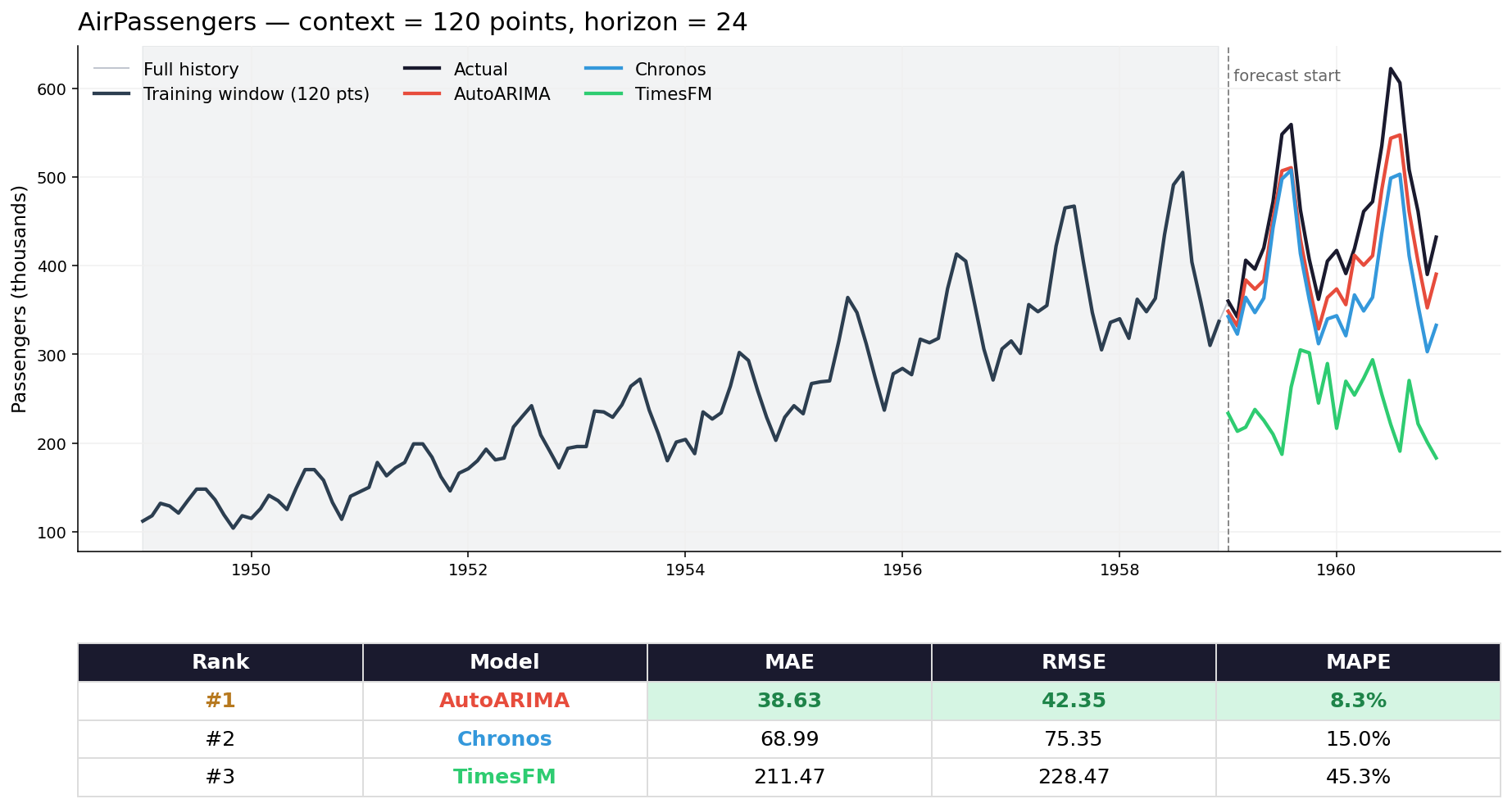
AirPassengers — full context (120 pts)

ARIMA is tuned for this: log transform + season_length=12. It wins.
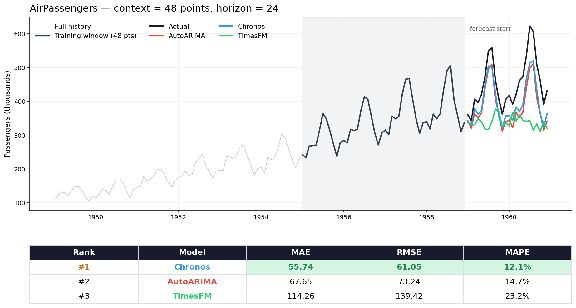
AirPassengers — shrink the window to 48 pts

Less history means ARIMA has less to fit. The gap narrows.
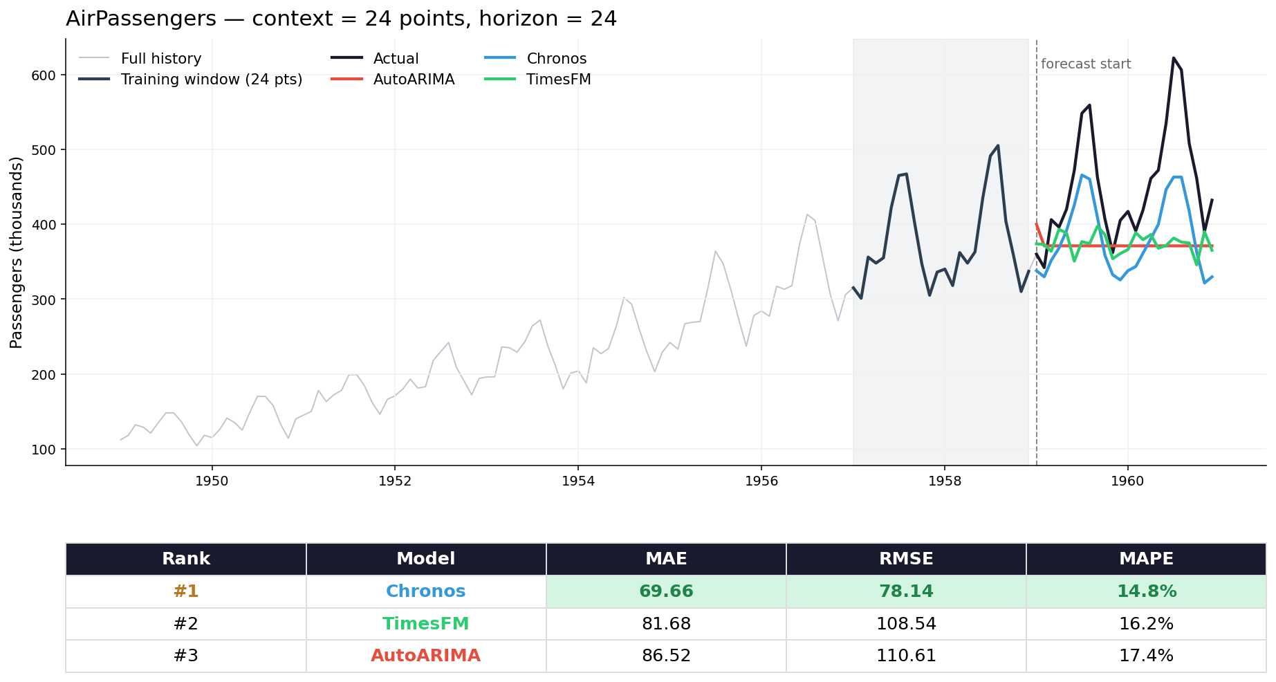
AirPassengers — just 24 pts of context

ARIMA drops to last. Chronos wins zero-shot — the FM's prior on seasonal data does more than ARIMA can with two years of history.
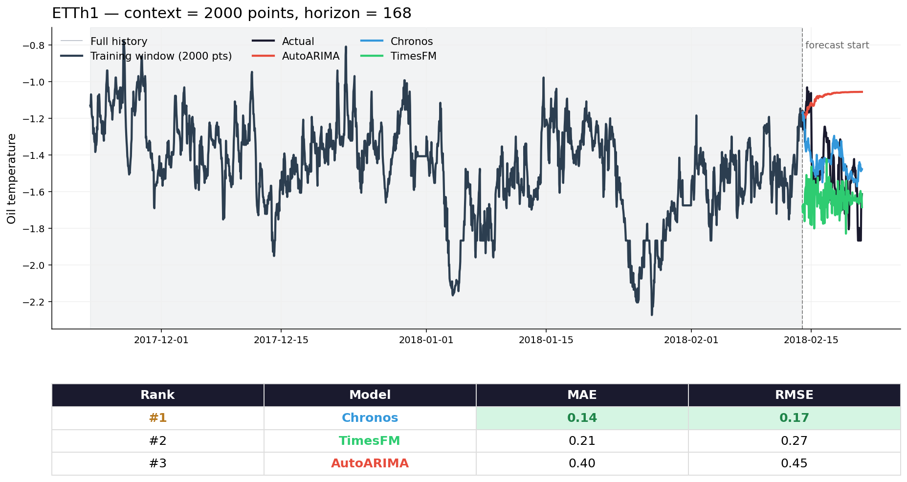
ETTh1 — messy, real-world hourly data (ctx = 2000)

Even with 2000 points of history, ARIMA only learns the local mean. Chronos halves the error.
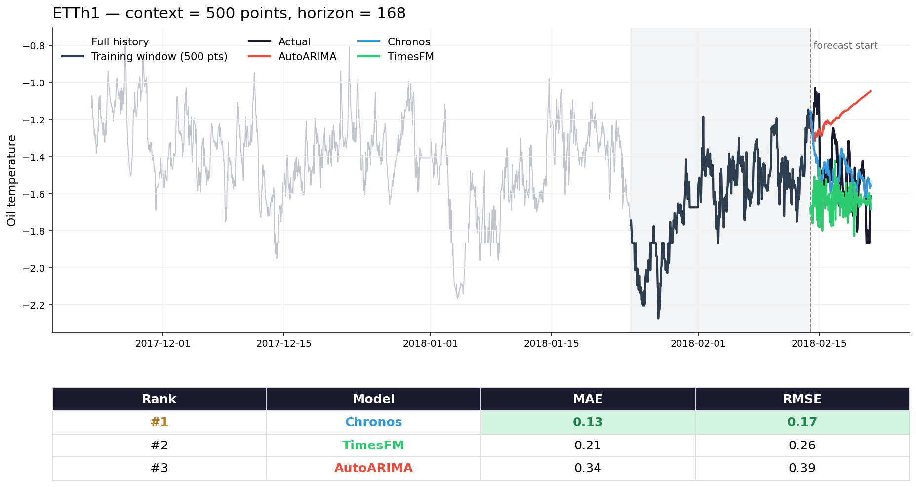
ETTh1 — shrink the window to 500 pts

FMs barely flinch (0.13 MAE). ARIMA still ~3× worse.
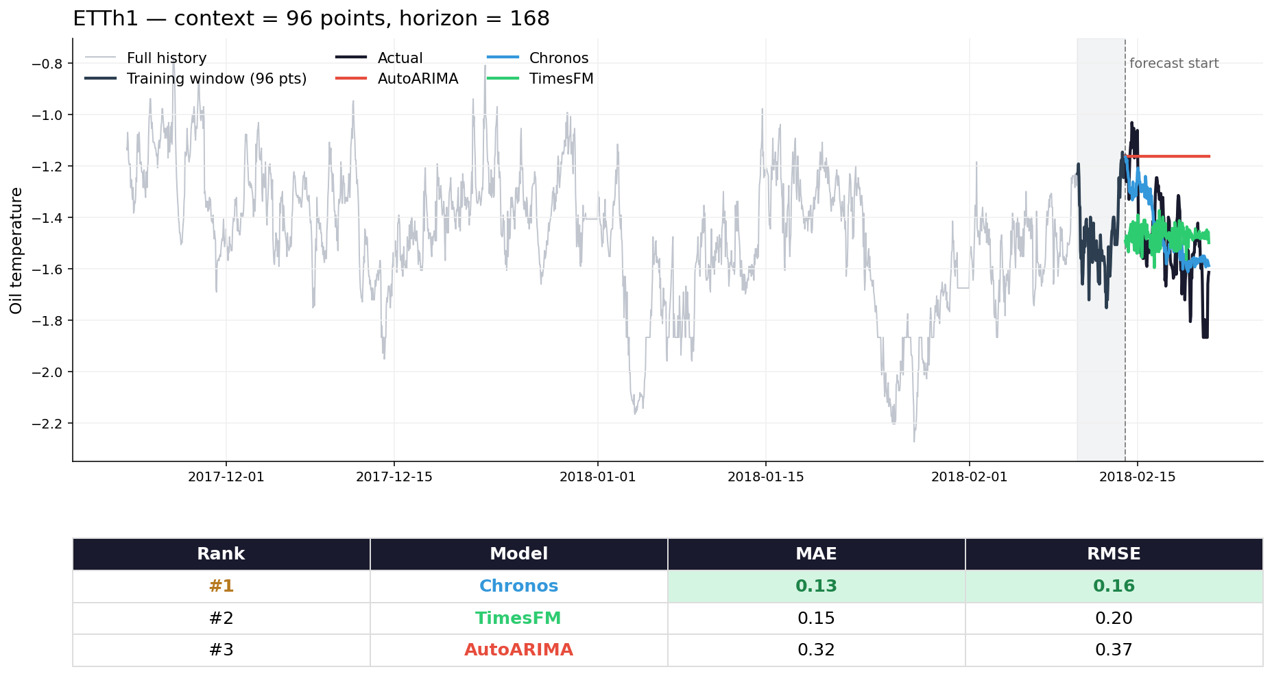
ETTh1 — just 96 pts (4 days) of context

Forecasting a week from 4 days of history. FMs still produce structured predictions with the same 0.13 MAE — zero-shot, unchanged.
Takeaways

What the demo showed — and what to do about it

What the demo showed

AirPassengers — famous, well-behaved

ARIMA wins (8.3% MAPE). But it had domain knowledge — log transform, season length 12. The FMs had zero tuning.

ETTh1 — unfamiliar hourly temperatures

Chronos halves ARIMA's error (0.13 vs 0.40 MAE). ARIMA goes flat; the FM picks up structure it has never seen.

On familiar, tuned data: ARIMA often wins. On new data: FMs give you a strong baseline in minutes instead of days.

When to use them

Good fit
  • Zero-shot on new datasets
  • Rapid prototyping — baseline in minutes
  • No ML team available — 3 lines of code
  • Many diverse series to forecast
  • Probabilistic forecasts out of the box
Bad fit
  • Known physics — domain equations beat black boxes
  • Need interpretability — stakeholders want the why
  • Complex multivariate — support is still maturing
  • Edge / real-time — ARIMA runs in ms
  • Highly specialized data far from training distribution

Best strategy: use FMs as a strong baseline. Compare against your tuned models, fine-tune if promising — don't choose, use both.

4 things to remember

Pre-train once, use everywhere

The paradigm shift that transformed NLP and vision has arrived for time series.

Transformers are the backbone

Same architecture as ChatGPT, adapted through patching or tokenization.

It runs on your laptop

Chronos is ~46M params, GPT-4 is ~1.7T — 37,000× smaller. Patterns in numbers are simpler than human language.

They won't replace expertise

But they dramatically lower the bar for good-enough forecasts on unfamiliar data.

You don't need to "know" that Paris is in France to forecast energy demand.

Try it yourself

# Install and try in 5 minutes
pip install chronos-forecasting

# Or try Google's approach
pip install timesfm

# Or the API route (no ML needed)
pip install nixtla # TimeGPT

All models on HuggingFace. All run on CPU. No GPU required.

Thank you

Everything is available here — slides, code, and app:

github.com/pigna90/talk-time-series-foundation-models

Questions?